1. Enter the scores in one of the columns on the Excel spreadsheet (see the example below). After the data has been entered, place the cursor where you wish to have the mean (average) appear and click the mouse button. Now move the cursor to the Function Wizard (fx) button and click on it.

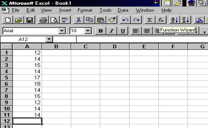
2. A dialog box will appear. Click on Statistical from the left section of the box and AVERAGE on the right section. After you have made those two selections, click on Next> at the bottom of the dialog box.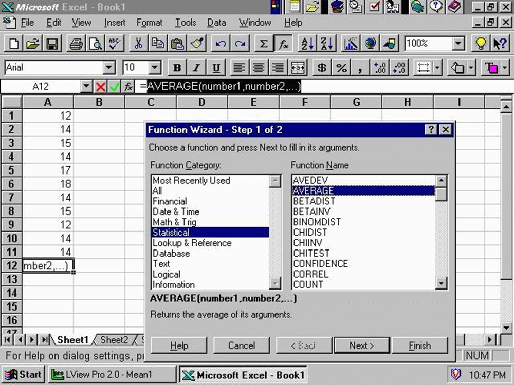

3. Enter the cell range for your list of numbers in the number 1 box. For example, if your data were in column A from row 1 to 11, you would enter A1:A11. Instead of typing the range, you can also move the cursor to the beginning of the set of scores you wish to use and click and drag the cursor across them. Once you have entered the range for your list, click on Finish at the bottom of the dialog box.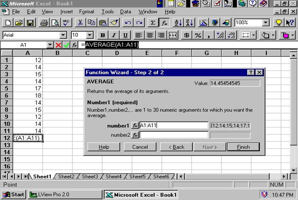

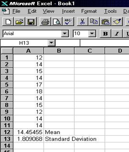
4. The mean (average) for the list will appear in the cell you selected.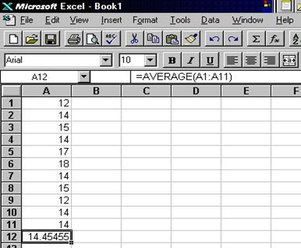

5. Place the cursor where you wish to have the standard deviation appear and click the mouse button. Now move the cursor to the Function Wizard (fx) button and click on it.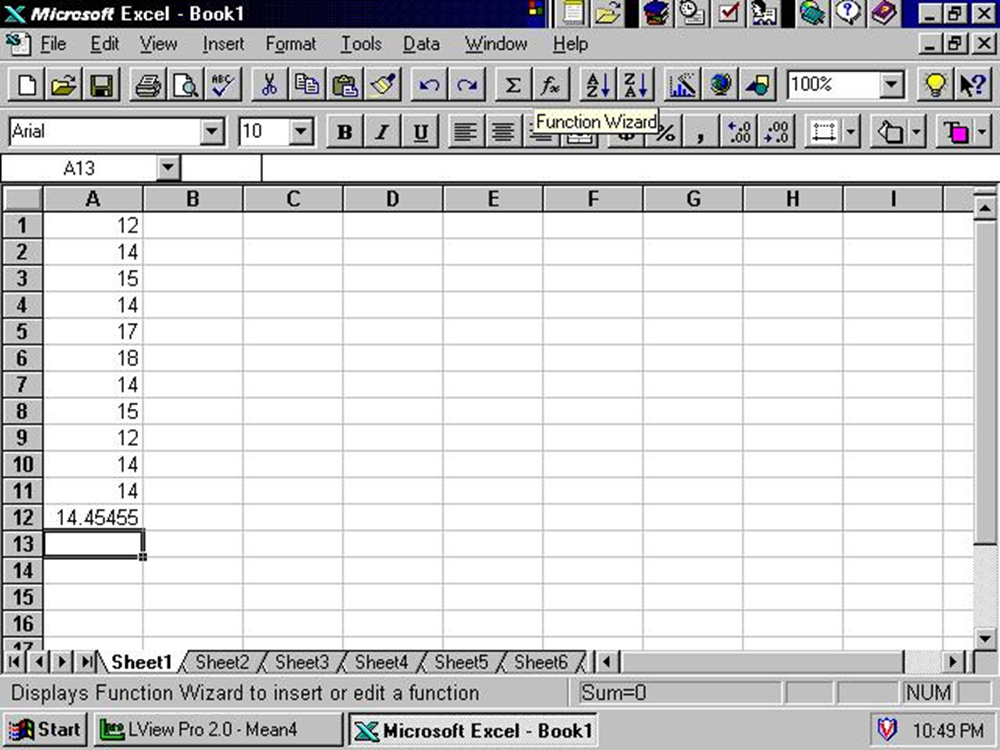

6. A dialog box will appear. Click on Statistical from the left section of the box and STDEV (for a sample) on the right section (Note: If your data is from a population, click onSTDEVP). After you have made your selections, click on Next> at the bottom of the dialog box.

7. Enter the cell range for your list of numbers in the number 1 box. For example, if your data were in column A from row 1 to 11, you would enter A1:A11. Instead of typing the range, you can also move the cursor to the beginning of the set of scores you wish to use and click and drag the cursor across them. Once you have entered the range for your list, click on Finish at the bottom of the dialog box.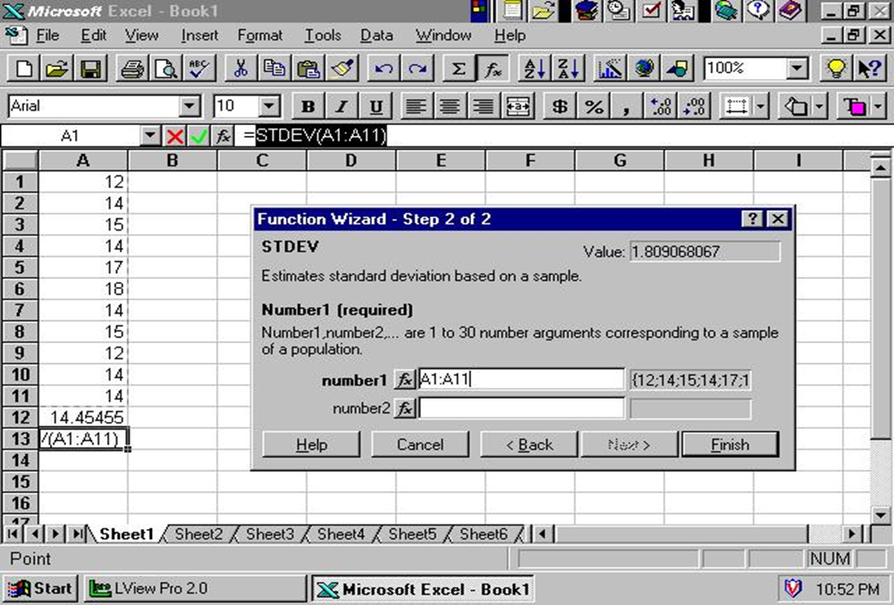

8. The standard deviation for the list will appear in the cell you selected.